LabPlot/ComputationalNotebooks
LabPlot/ComputationalNotebooks
Introduction
LabPlot's Computational Notebooks offer an interactive interface to various open-source mathematics and statistics packages as well as programming languages. These include Maxima, Octave, R, Scilab, Sage, KAlgebra, Qalculate!, Python, Julia, and Lua. This integration enables execution of computations and immediate visualization of results within the same environment, providing a user-friendly interface for complex calculations and data analysis.
As a brief introduction, see the video on how to use Computational Notebooks in LabPlot.
Prerequisites
To make use of the notebook interface for a specific language, it needs to be installed first. For systems like Maxima, Octave, Sage and Scilab, the communication is happening with the executable of this system and it's enough to point LabPlot in the application settings to its location if its not found automatically:
For R, Python and Julia the interpreter is embedded into LabPlots process and only those versions of these languages can be used that were used on the build system during the build time of LabPlot. For which versions to use we refer to the FAQ
On Windows and on macOS (starting with LabPlot 2.12) all languages mentioned above are supported except of R, Lua, Julia and Qalculate!. On Linux, the support for the different languages is determined by the build and package step of the distribution in use.
Basic Concepts
- Multi-Language and CAS Support: LabPlot supports a wide range of programming languages and CAS, empowering users to utilize the computational capabilities of Maxima, Octave, R, Scilab, Sage, KAlgebra, Qalculate!, Python, Julia, and Lua within the same notebook.
- Simultaneous Notebooks and Languages: Users can work with multiple notebooks and languages simultaneously, facilitating a flexible workflow adaptable to various computational requirements.
- Array-like Data as Plot Sources: LabPlot recognizes notebook variables containing array-like data (e.g., Maxima lists, Python lists and tuples, Julia vectors and tuples) and permits selecting them as sources for interactive plots, simplifying plot creation by utilizing computation outputs directly.
- Extensive Edition Capabilities: The notebook interface offers extensive editing capabilities, enabling users to perform complex manipulations and analyses on their data directly within the notebook.
- Plotting Support: LabPlot provides robust support for plotting, enabling users to create a wide range of plots and charts directly within the notebook interface.
- Markdown and LaTeX Syntax: Users can utilize Markdown and LaTeX syntax within the notebooks to create richly formatted text, equations, and documentation alongside their computations and visualizations.
- Compatibility with Jupyter and Cantor Projects: LabPlot can read Jupyter and Cantor projects, allowing users to import and work with notebooks created in these environments.
- Syntax Highlighting: The notebook interface features syntax highlighting, enhancing code readability and writability by distinguishing different parts of the code syntax.
- Integrated Help: LabPlot offers integrated help for CAS systems and programming languages, including features for downloading, searching, and navigating documentation, facilitating user learning and utilization of underlying system features.
Working with Computational Notebooks
- Launching a Notebook: To begin, users select the desired programming language or CAS from within LabPlot, opening a new notebook interface where they can write and execute code.
- Executing Code: Code execution is straightforward; users can select code and press the execution button or use a keyboard shortcut to run the code. The computation results are displayed directly below the executed code, facilitating immediate visualization and analysis.
- Visualizing Data: After performing calculations, users can select the output variables as sources for plots within the notebook interface. LabPlot automatically recognizes array-like data structures from supported languages, simplifying plot creation.
- Data Manipulation: Within the notebook, users can manipulate data using the syntax and functions of the chosen programming language. This includes filtering, sorting, aggregating, and transforming data before visualization.
- Saving and Sharing: Notebooks can be saved in the LabPlot project file format, facilitating easy sharing and collaboration. Users can also export notebooks to various formats for use in other applications or for sharing with others.
Properties Panels
General
Table of Contents
Help
Variables
Documentation
Visualization in LabPlot
While it is possible to visualize the data directly in the notebooks for most of the supported systems, sometimes it is desired to visualize the results of computations that were performed in a notebook directly in LabPlot's Worksheet. This is useful for example when the results need to be visualized together with other data imported into LabPlot or when the more advanced and interactive styling and navigation capabilities are required.
To enable this, LabPlot recognizes the creation of variables holding array-like data and allows to select them as a data source for plots and analysis functions similarly to the columns in a Spreadsheet. The currently supported data containers are:
- Maxima lists
- Python lists, tuples and NumPy arrays
- Julia vectors and tuples
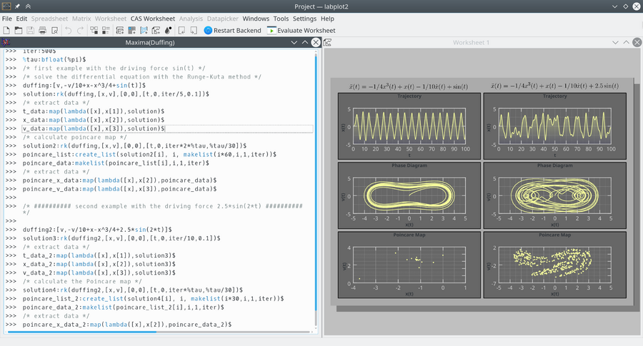
The examples below show how powerful calculations carried out inside of different environments can be combined with the user-friendly visualization and editing capabilities of LabPlot. In the first example, a Maxima session exploring the chaotic dynamics of the Duffing oscillator is shown. The forced oscillator's differential equation is solved using Maxima, and the results are visualized using LabPlot. Plots include the oscillator's trajectory, phase space, and Poincaré map, showcasing the system's complex behavior.

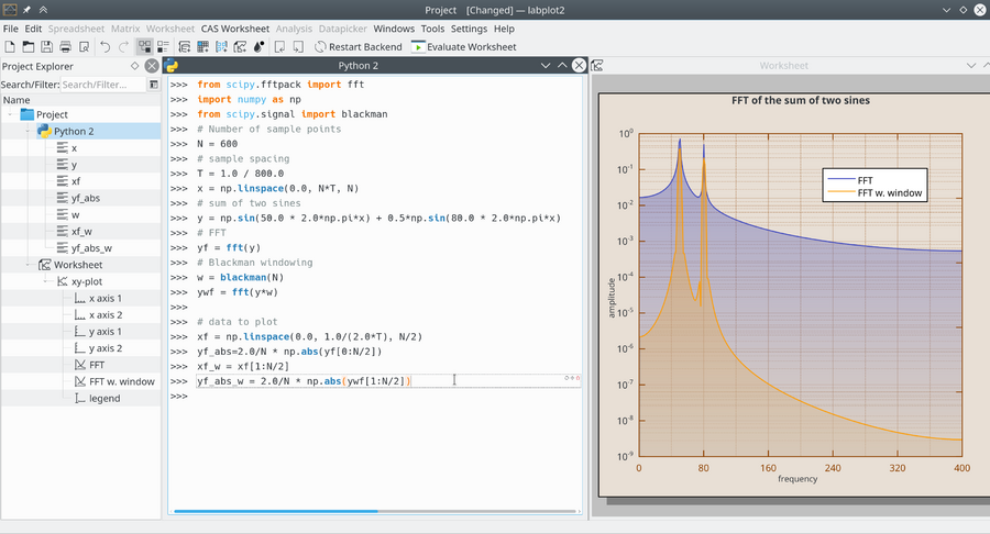
In a second example, Python session analyzing the effect of Blackman windowing on the Fourier transform is shown. It demonstrates how windowing can enhance the clarity of frequency components in signal processing, with plots showing the Fourier transform before and after applying the Blackman window.

