KmPlot/Using Sliders: Difference between revisions
Appearance
Pipesmoker (talk | contribs) No edit summary |
m fix typos |
||
| (7 intermediate revisions by 2 users not shown) | |||
| Line 1: | Line 1: | ||
<languages /> | <languages /> | ||
<translate> | <translate> | ||
A main feature | <!--T:1--> | ||
A main feature of '''KmPlot''' is to visualize the influence of parameters to the curve of a function. | |||
==Moving a Sinus Curve== | ==Moving a Sinus Curve== <!--T:2--> | ||
<!--T:3--> | |||
Let's see, how to move a sinus curve left and right: | Let's see, how to move a sinus curve left and right: | ||
* Create a new | <!--T:4--> | ||
* Create a new Cartesian plot. | |||
* Enter the equation {{Input|1=f(x,a) = sin(x-a)}} | * Enter the equation {{Input|1=f(x,a) = sin(x-a)}} | ||
* Check the <menuchoice>Slider</menuchoice> option and choose <menuchoice>Slider No. 1</menuchoice> from the drop down list. | * Check the <menuchoice>Slider</menuchoice> option and choose <menuchoice>Slider No. 1</menuchoice> from the drop down list. | ||
* To make the available sliders visible, check <menuchoice>View -> Show Sliders</menuchoice> | * To make the available sliders visible, check <menuchoice>View -> Show Sliders</menuchoice> | ||
<!--T:5--> | |||
Now you can move the slider and see how the parameter value modifies the position of the curve. | Now you can move the slider and see how the parameter value modifies the position of the curve. | ||
<!--T:7--> | |||
<gallery perrow="3" caption="Screenshots"> | |||
<gallery perrow="3"> | |||
Image:Kmplot_function_with_param.png|Input | Image:Kmplot_function_with_param.png|Input | ||
Image:Kmplot_view_show_sliders.png|Show sliders option | Image:Kmplot_view_show_sliders.png|Show sliders option | ||
| Line 22: | Line 25: | ||
</gallery> | </gallery> | ||
==Trajectory of a Projectile== | ==Trajectory of a Projectile== <!--T:8--> | ||
<!--T:13--> | |||
Now let's have a look at the maximum distance of a projectile thrown with different angles. We use a parametric plot depending on an additional parameter which is the | Now let's have a look at the maximum distance of a projectile thrown with different angles. We use a parametric plot depending on an additional parameter which is the angle. | ||
* Define a | <!--T:10--> | ||
* Define a constant v_0 for the starting velocity. | |||
* Create a new parametric plot | * Create a new parametric plot | ||
* Enter the equations {{Input|1=<nowiki>f_x(t,α) = v_0∙cos(α)∙t | * Enter the equations {{Input|1=<nowiki>f_x(t,α) = v_0∙cos(α)∙t | ||
f_y(t,α) =2+ v_0∙sin(α)∙t−5∙t^2</nowiki>}} | f_y(t,α) = 2+v_0∙sin(α)∙t−5∙t^2</nowiki>}} | ||
* Check the <menuchoice>Slider</menuchoice> option and choose <menuchoice>Slider No. 1</menuchoice> from the drop down list. | * Check the <menuchoice>Slider</menuchoice> option and choose <menuchoice>Slider No. 1</menuchoice> from the drop down list. | ||
* To make the available sliders visible, check <menuchoice>View -> Show Sliders</menuchoice> | * To make the available sliders visible, check <menuchoice>View -> Show Sliders</menuchoice> | ||
<!--T:11--> | |||
Now you can move the slider and see how the distance depends on the parameter value. | Now you can move the slider and see how the distance depends on the parameter value. | ||
<!--T:14--> | |||
[[Image:Kmplot_projectile.gif|center|692px|]] | |||
<!--T:12--> | |||
[[Category:Education]] | [[Category:Education]] | ||
</translate> | </translate> | ||
Latest revision as of 18:08, 11 October 2010
A main feature of KmPlot is to visualize the influence of parameters to the curve of a function.
Moving a Sinus Curve
Let's see, how to move a sinus curve left and right:
- Create a new Cartesian plot.
- Enter the equation
f(x,a) = sin(x-a)
- Check the option and choose from the drop down list.
- To make the available sliders visible, check
Now you can move the slider and see how the parameter value modifies the position of the curve.
- Screenshots
-
Input
-
Show sliders option
-
Slider window
Trajectory of a Projectile
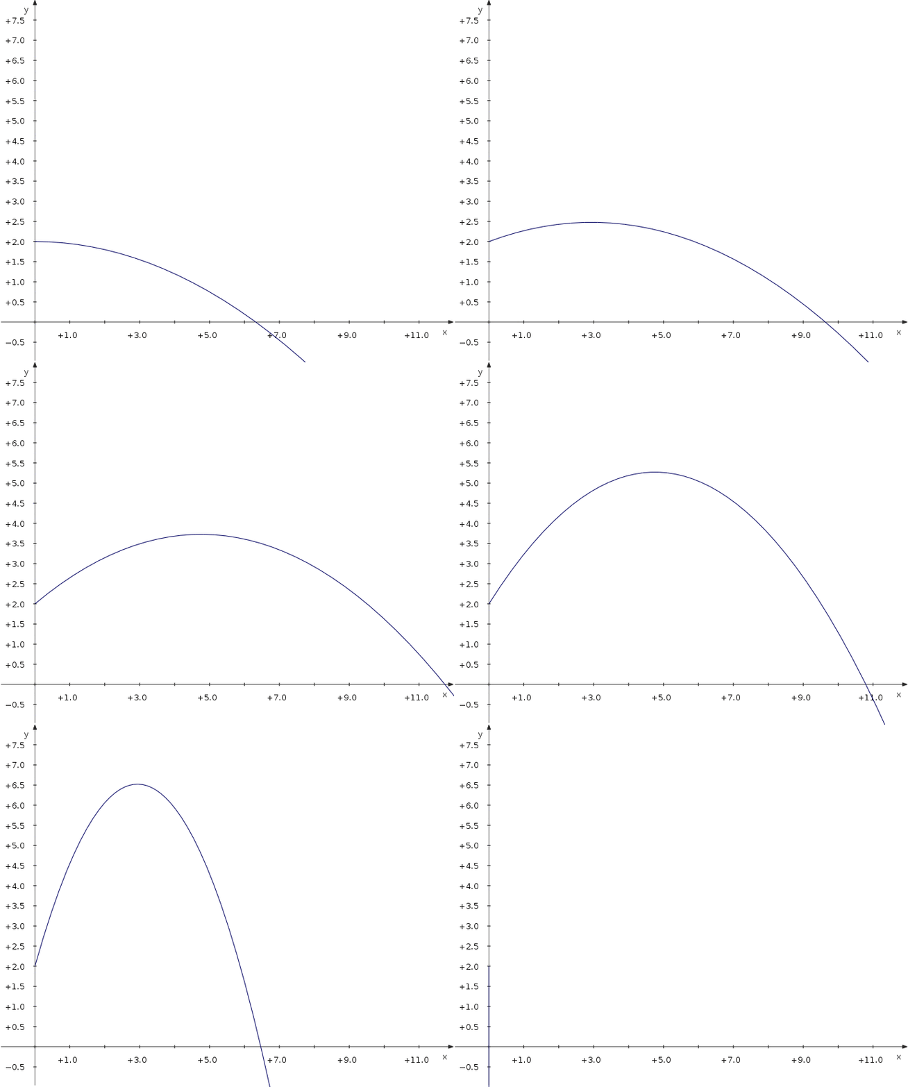
Now let's have a look at the maximum distance of a projectile thrown with different angles. We use a parametric plot depending on an additional parameter which is the angle.
- Define a constant v_0 for the starting velocity.
- Create a new parametric plot
- Enter the equations
f_x(t,α) = v_0∙cos(α)∙t
f_y(t,α) = 2+v_0∙sin(α)∙t−5∙t^2
- Check the option and choose from the drop down list.
- To make the available sliders visible, check
Now you can move the slider and see how the distance depends on the parameter value.


